Preparation
For this example geodata is joined with municipality level data from Statistics Finland. Load packages which are needed for data wrangling and plotting. For ternary color coded maps we are using tricolore packgage. Check more information of tricolore package in github https://github.com/jschoeley/tricolore. Other special package for spatial data we need is geofi package, which download spatial data from Statistics Finland’s geoserver.
# remotes::install_github("ropengov/geofi")
library(geofi)
#>
#> geofi R package: tools for open GIS data for Finland.
#> Part of rOpenGov <ropengov.github.io>.
# install.packages("tricolore")
library(tricolore)
#> Registered S3 methods overwritten by 'ggtern':
#>   method           from
#>   grid.draw.ggplot ggplot2
#>   plot.ggplot      ggplot2
#>   print.ggplot     ggplot2
library(dplyr)
#>
#> Attaching package: 'dplyr'
#> The following objects are masked from 'package:stats':
#>
#>     filter, lag
#> The following object is masked from '.env':
#>
#>     n
#> The following objects are masked from 'package:base':
#>
#>     intersect, setdiff, setequal, union
library(tidyr)
library(ggplot2)
Download and prepare datasets
# Download municipalities geodata
municipalities17 <- get_municipalities(year = 2017)
#> Requesting response from: http://geo.stat.fi/geoserver/wfs?service=WFS&version=1.0.0&request=getFeature&typename=tilastointialueet%3Akunta4500k_2017
#> Warning: Coercing CRS to epsg:3067 (ETRS89 / TM35FIN)
#> Data is licensed under: Attribution 4.0 International (CC BY 4.0)

# Pull municipalities and population data from Statistics Finland
library(pxweb)
#> pxweb: R tools for PX-WEB API.
#> Copyright (C) 2014-2018 Mans Magnusson, Leo Lahti et al.
#> https://github.com/ropengov/pxweb
pxweb_query_list <- list("Alue 2019"=c("020","005","009","010","016","018","019","035","043","046","047","049","050","051","052","060","061","062","065","069","071","072","074","075","076","077","078","079","081","082","086","111","090","091","097","098","099","102","103","105","106","108","109","139","140","142","143","145","146","153","148","149","151","152","165","167","169","170","171","172","176","177","178","179","181","182","186","202","204","205","208","211","213","214","216","217","218","224","226","230","231","232","233","235","236","239","240","320","241","322","244","245","249","250","256","257","260","261","263","265","271","272","273","275","276","280","284","285","286","287","288","290","291","295","297","300","301","304","305","312","316","317","318","398","399","400","407","402","403","405","408","410","416","417","418","420","421","422","423","425","426","444","430","433","434","435","436","438","440","441","475","478","480","481","483","484","489","491","494","495","498","499","500","503","504","505","508","507","529","531","535","536","538","541","543","545","560","561","562","563","564","309","576","577","578","445","580","581","599","583","854","584","588","592","593","595","598","601","604","607","608","609","611","638","614","615","616","619","620","623","624","625","626","630","631","635","636","678","710","680","681","683","684","686","687","689","691","694","697","698","700","702","704","707","729","732","734","736","790","738","739","740","742","743","746","747","748","791","749","751","753","755","758","759","761","762","765","766","768","771","777","778","781","783","831","832","833","834","837","844","845","846","848","849","850","851","853","857","858","859","886","887","889","890","892","893","895","785","905","908","911","092","915","918","921","922","924","925","927","931","934","935","936","941","946","976","977","980","981","989","992"),
       "Tiedot"=c("M411", "M391","M421","M478"),
       "Vuosi"=c("2017"))
px_data <- pxweb_get(url = "http://pxnet2.stat.fi/PXWeb/api/v1/fi/Kuntien_avainluvut/2019/kuntien_avainluvut_2019_aikasarja.px",
                     query = pxweb_query_list)

# Convert to data.frame and wrangle dataset so that every row is municipality
tk_data <- as.data.frame(px_data,
                         column.name.type = "text",
                         variable.value.type = "text")
tk_data <- tk_data %>%
  rename(name = `Alue 2019`) %>%
  mutate(name = as.character(name),
         # Paste Tiedot and Vuosi
         Tiedot = paste(Tiedot, Vuosi)) %>%
  select(-Vuosi) %>%
  spread(Tiedot, `Kuntien avainluvut`) %>%
  as_tibble()
tk_data <- janitor::clean_names(tk_data)

# Rename variables in english
tk_data <- tk_data %>%
  rename(
    under_15 = alle_15_vuotiaiden_osuus_vaestosta_percent_2017,
    y16_64 = x15_64_vuotiaiden_osuus_vaestosta_percent_2017,
    over64 = yli_64_vuotiaiden_osuus_vaestosta_percent_2017,
    popu2017 = vakiluku_2017
  )


# Join with Statistics Finland attribute data
dat <- left_join(municipalities17, tk_data)
#> Joining, by = "name"

# Join the municipality level data with internal municipality_key_2017-data
finland_popu2017 <- left_join(dat, municipality_key_2017, by = c("name" = "name_fi"))
Calculating color-code to the dataset
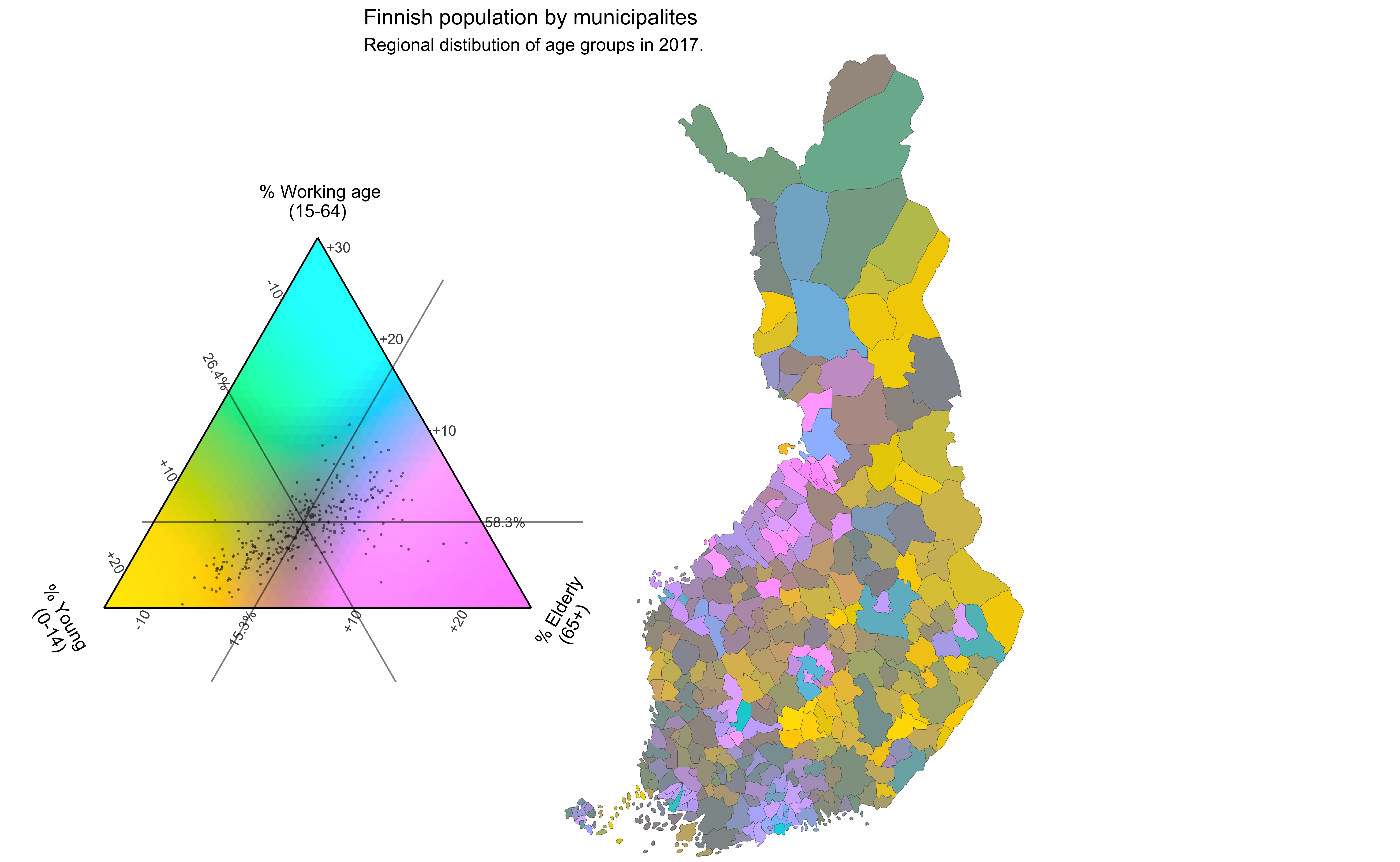
Ternary color codes are calculated by Tricolore()-function, which excepts variables which is used for color coding. Save rgb values to population dataset.
tric_dat <- Tricolore(finland_popu2017,
                      p1 = 'over64',
                      p2 = 'y16_64',
                      p3 = 'under_15',
                      center = NA,
                      crop = TRUE
                      )
#> Warning: Ignoring unknown aesthetics: z
finland_popu2017$popu_rgb <- tric_dat$rgb
Plot map by ggplot and use scale_fill_identity() option to make sure that each region is color coded by rgb-code.
plot_pop <- ggplot(finland_popu2017) +
  geom_sf(aes(fill = popu_rgb, geometry = geom), size = .1) +
  scale_fill_identity()
plot_pop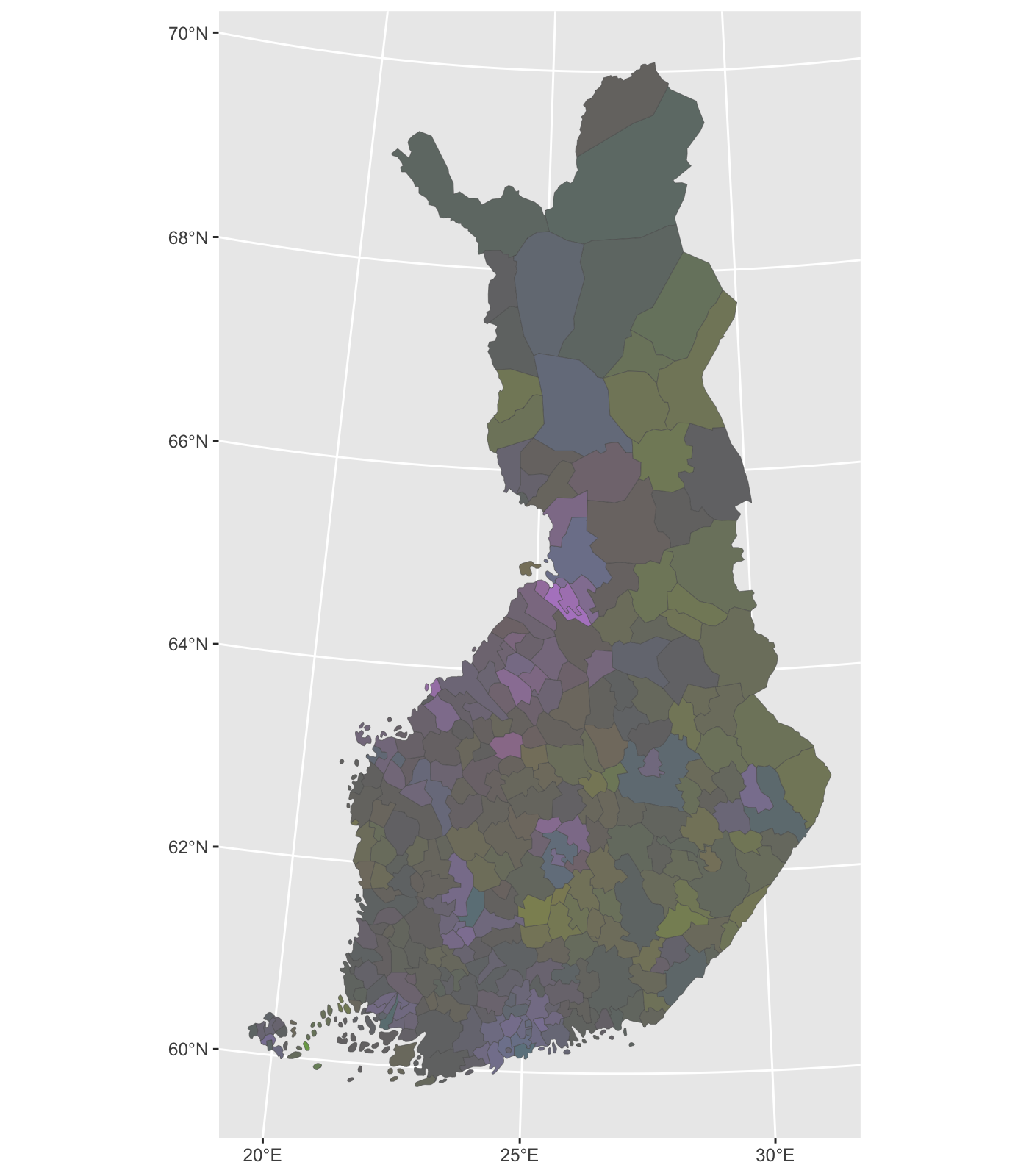
Ternary colors can be adjusted to distinct municipalies differences better.
tric_dat <- Tricolore(finland_popu2017,
                      p1 = 'over64',
                      p2 = 'y16_64',
                      p3 = 'under_15',
                      center = NA,
                      crop = TRUE,
                      spread = 3,
                      contrast = .4,
                      lightness = 1,
                      chroma = 1,
                      hue = 2/12
                      )
#> Warning: Ignoring unknown aesthetics: z
finland_popu2017$popu_rgb <- tric_dat$rgb
plot_pop <- ggplot(finland_popu2017) +
geom_sf(aes(fill = popu_rgb, geometry = geom), size = .1) +
scale_fill_identity()
plot_pop
Building legend for a plot
Legend for tertinary color is added by ggtern and annotation_custom(). Package ggtern is important to load afer ggplot2 package.
library(ggtern)
#> --
#> Remember to cite, run citation(package = 'ggtern') for further info.
#> --
#>
#> Attaching package: 'ggtern'
#> The following objects are masked from 'package:ggplot2':
#>
#>     aes, annotate, ggplot, ggplot_build, ggplot_gtable, ggplotGrob,
#>     ggsave, layer_data, theme_bw, theme_classic, theme_dark,
#>     theme_gray, theme_light, theme_linedraw, theme_minimal, theme_void
plot_pop <- ggplot(finland_popu2017) +
  geom_sf(aes(fill = popu_rgb, geometry = geom), size = .1) +
  scale_fill_identity() +
  coord_sf(xlim = c(-2e5,7.5e5), ylim = c(66.3e5, 77.7e5), expand = FALSE, datum = NA) +
  annotation_custom(
    ggplotGrob(tric_dat$key + labs(L = "% Young\n(0-14)", T = " % Working age\n(15-64)", R = "% Elderly\n(65+)")) ,
    xmin = -7e5, xmax = 1.7e5, ymin = 68e5, ymax = 77e5
  ) +
  theme_void() +
  ggtitle("Finnish population by municipalites",
       subtitle = "Regional distibution of age groups in 2017.")
#> Coordinate system already present. Adding new coordinate system, which will replace the existing one.

  # labs(title = "Finnish population by municipalites",
  #      subtitle = "Regional distibution of age groups in 2017.",
  #      caption = "Data by Statistics Finland")
plot_pop